A transistor amplifier: bias, gain, noise and clipping

The results on this page were computed when the vignette was written (see vignettes/precompile.R); the code is what produced them.

library(spice)

One deck, four analyses: a common-emitter stage with an emitter bypass, looked at the way a designer would — where it sits, how much it amplifies and up to where, how much noise it adds, and what it does to a signal that is too large.

The circuit

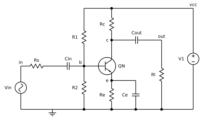
amp <- "common-emitter amplifier
vcc vcc 0 12
vin in 0 dc 0 ac 1 sin(0 10m 1k)
rs in b1 1k
cin b1 b 10u
r1 vcc b 47k
r2 b 0 10k
q1 c b e qn
rc vcc c 4.7k
re e 0 1k
ce e 0 100u
cout c out 10u
rl out 0 10k
.model qn npn(is=1e-14 bf=200 vaf=100 cje=4p cjc=2p tf=0.3n rb=50)
.op
.ac dec 20 1 100meg
.noise v(out) vin dec 10 10 1meg
.tran 10u 4m
.end"
res <- spice_run(amp)
res
#> <spice_result> common-emitter amplifier
#> 5 plots:
#> • Operating Point: 9 variables x 1 point, real
#> • AC Analysis: 10 variables x 161 points, complex, scale frequency
#> • Noise Spectral Density Curves: 3 variables x 51 points, real, scale frequency
#> • Integrated Noise: 2 variables x 1 point, real
#> • Transient Analysis: 10 variables x 408 points, real, scale time

Bias

spice_op() gives the operating point as a named vector.

res |> spice_op(c("b", "e", "c"))
#>     v(b)     v(c)     v(e) 
#> 2.050245 5.510875 1.387337

The collector sits near mid-supply, with about 1.4 mA through the transistor (v(e) across the 1 kOhm emitter resistor).

Gain and bandwidth

The AC plot is complex; its tidy table carries the magnitude, the gain in dB and the phase in degrees. .measure expressions work on a finished plot too, through spice_measure().

out <- res |> spice_tidy("ac", "out")

ggplot(out, aes(scale, db)) +
  geom_line(colour = "#b8741a", linewidth = 0.8) +
  scale_x_log10() +
  labs(x = "frequency (Hz)", y = "gain (dB)", title = "Voltage gain, v(out)/vin")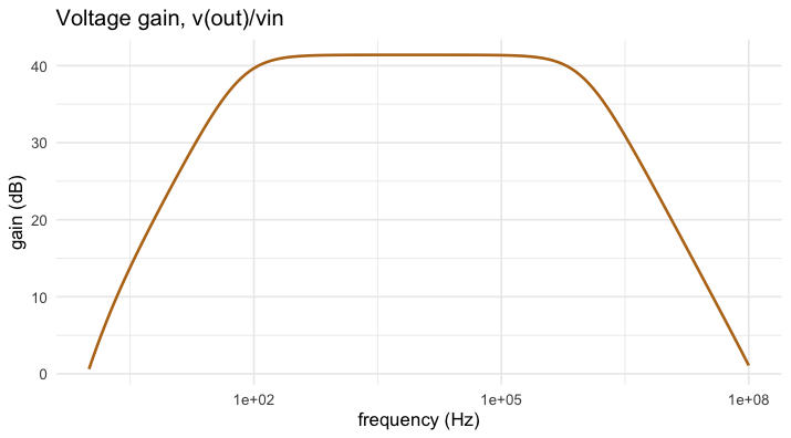

plot of chunk ac

acp <- spice_plots(res)[["AC Analysis"]]
m <- spice_measure(acp, c(
  peak = "max vdb(out)",
  f_lo = "when vdb(out)=38.4 rise=1",
  f_hi = "when vdb(out)=38.4 fall=1"
))
m[, c("name", "value")]
#> # A tibble: 3 × 2
#>   name     value
#>   <chr>    <dbl>
#> 1 peak      41.4
#> 2 f_lo      70.4
#> 3 f_hi  987170.

About 41 dB in the passband; the lower corner is set by the emitter bypass capacitor, the upper one by the transistor’s capacitances against the source resistance.

Noise

.noise gives the output noise density and the same referred to the input, and their integrals over the sweep.

nz <- spice_tidy(res, "noise")
ggplot(nz, aes(scale, value * 1e9, colour = variable)) +
  geom_line(linewidth = 0.8) +
  scale_x_log10() + scale_y_log10() +
  labs(x = "frequency (Hz)", y = "noise density (nV/sqrt(Hz))", colour = NULL)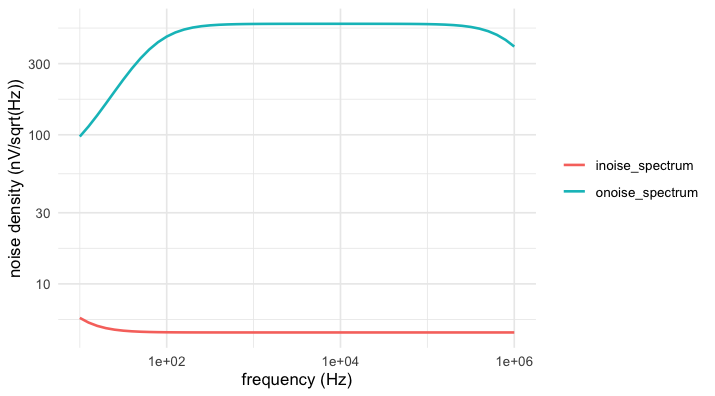

plot of chunk noise

spice_tidy(res, "inoise")[, c("variable", "value")]
#> # A tibble: 2 × 2
#>   variable             value
#>   <chr>                <dbl>
#> 1 v(onoise_total) 0.000490  
#> 2 v(inoise_total) 0.00000484

A signal that is too large

The deck’s transient drives 10 mV; the stage is linear there. Sixty millivolts is another matter. A session keeps the circuit built and lets one alter a source and run again.

s <- spice_session(amp)
run_at <- function(amplitude) {
  spice_alter(s, "vin", sin = c(0, amplitude, 1e3))
  tr <- spice_rerun(s) |> spice_tidy("tran", "out")
  tr <- tr[, c("scale", "value")]
  tr$drive <- sprintf("%g mV", amplitude * 1e3)
  tr
}
both <- rbind(run_at(10e-3), run_at(60e-3))

ggplot(both, aes(scale * 1e3, value, colour = drive)) +
  geom_line(linewidth = 0.7) +
  labs(x = "time (ms)", y = "v(out) (V)", colour = "input",
       title = "The stage clips on the way down")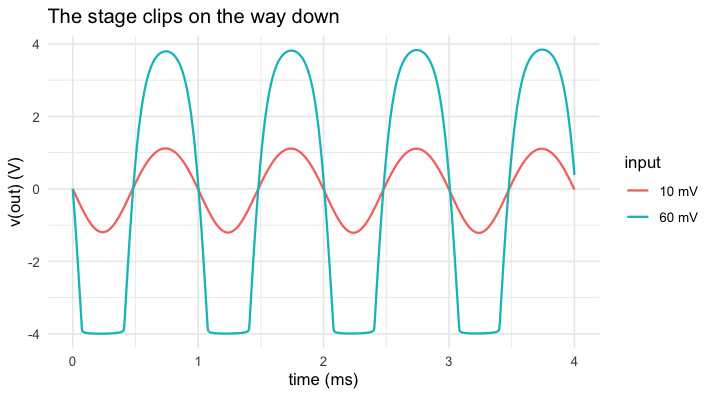

plot of chunk clip