Transmission lines and reflections

The results on this page were computed when the vignette was written (see vignettes/precompile.R); the code is what produced them.

library(spice)

A wire becomes a transmission line when the signal’s edge is shorter than the trip along it. Then what arrives depends on what the line is terminated with, and a mismatch sends part of the wave back.

A mismatched line

A 50 ohm line, 4.38 ns long, driven through 10 ohm into a 1 kOhm load: mismatched at both ends, so the 1 ns edge bounces back and forth.

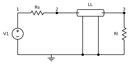
line <- function(rs, rl) sprintf("line
v1 1 0 pwl(0 0 1n 0 2n 1 100n 1)
rs 1 2 %g
o1 2 0 3 0 ll
rl 3 0 %g
.model ll ltra l=9.13e-9 c=3.65e-12 len=24
.tran 0.1n 60n
.end", rs, rl)

far <- function(res, label) {
  tr <- res |> spice_tidy("tran", "v(3)")
  tr <- tr[, c("scale", "value")]
  tr$case <- label
  tr
}
both <- rbind(
  far(spice_run(line(10, 1000)), "10 ohm source, 1 kOhm load"),
  far(spice_run(line(50, 50)), "matched: 50 ohm both ends")
)

ggplot(both, aes(scale * 1e9, value, colour = case)) +
  geom_line(linewidth = 0.7) +
  labs(x = "time (ns)", y = "far-end voltage (V)", colour = NULL,
       title = "The same edge, with and without matching") +
  theme(legend.position = "bottom")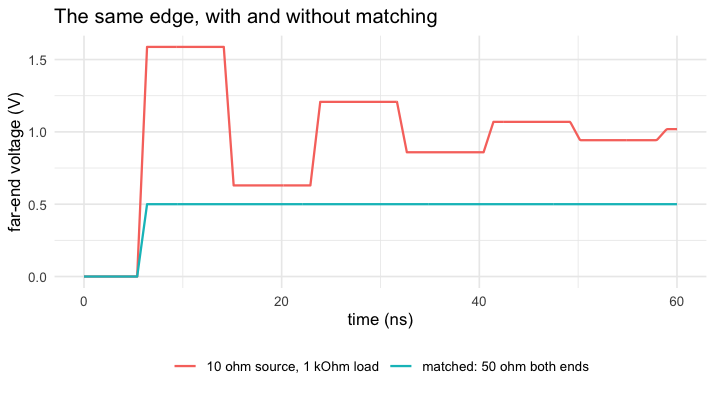

plot of chunk deck

Matched, the edge arrives once, at half the source’s amplitude, and that is the end of it. Mismatched, it overshoots to 1.6 V and rings for tens of nanoseconds.

How exact is it

A lossless line with resistive terminations has a closed form: the far end is a sum of delayed copies of the launched edge, each smaller by the product of the two reflection coefficients.

z0 <- sqrt(9.13e-9 / 3.65e-12)
td <- 24 * sqrt(9.13e-9 * 3.65e-12)
gs <- (10 - z0) / (10 + z0)
gl <- (1000 - z0) / (1000 + z0)
launched <- function(t) pmin(pmax(t - 1e-9, 0), 1e-9) / 1e-9 * z0 / (z0 + 10)
v3 <- function(t) {
  rowSums(sapply(0:11, function(k) (1 + gl) * (gl * gs)^k * launched(t - (2 * k + 1) * td)))
}
c(z0 = z0, delay_ns = td * 1e9, gamma_source = gs, gamma_load = gl)
#>           z0     delay_ns gamma_source   gamma_load 
#>   50.0136968    4.3811998   -0.6667427    0.9047371

worst <- function(options = NULL) {
  tr <- spice_run(line(10, 1000), options = options) |>
    spice_tidy("tran", "v(3)")
  max(abs(tr$value - v3(tr$scale)))
}
c(dune = worst(), spice3 = worst(list(compat = "spice3")))
#>        dune      spice3 
#> 0.001573332 0.010080671

In volts, on a 1 V edge. SPICE’s rule for where to put a timepoint when a corner of the wave arrives almost never fires, so the corner falls between timepoints and is rounded a little more at every bounce; Dune’s finds the corners. vignette("defaults") has the rest of that story.

A lossy line

Real interconnect has resistance. The same line with 0.2 ohm per unit length rounds the edges and lowers the plateaus — and no closed form is left to compare with.

lossy <- sub("l=9.13e-9", "r=0.2 l=9.13e-9", line(10, 1000), fixed = TRUE)
cmp <- rbind(
  far(spice_run(line(10, 1000)), "lossless"),
  far(spice_run(lossy), "0.2 ohm per unit length")
)
ggplot(cmp, aes(scale * 1e9, value, colour = case)) +
  geom_line(linewidth = 0.7) +
  labs(x = "time (ns)", y = "far-end voltage (V)", colour = NULL) +
  theme(legend.position = "bottom")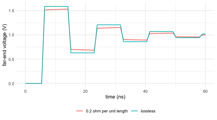

plot of chunk lossy