
spice runs SPICE3 netlists on Dune, a circuit simulator derived from Berkeley SPICE3f5, and hands the results back as tidy data. This vignette runs one deck end to end: a second-order RLC low-pass driven by a voltage step, with a transient and an AC analysis.
A deck
A deck is ordinary SPICE3 input. The first line is the title; the
analysis cards (.tran, .ac, …) say what to
compute. Here it is given as text; spice_run() equally
accepts the path of a .cir file.
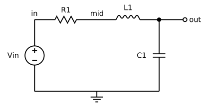
deck <- "RLC low-pass
vin in 0 pulse(0 1 0 1u) ac 1
r1 in mid 50
l1 mid out 1m
c1 out 0 1u
.tran 2u 1m
.ac dec 50 100 100k
.end"
Running it
res <- spice_run(deck)
res
#> <spice_result> RLC low-pass
#> 2 plots:
#> • Transient Analysis: 6 variables x 523 points, real, scale time
#> • AC Analysis: 6 variables x 151 points, complex, scale frequency
Each analysis produces a plot, named as SPICE3 names it in a rawfile.
Simulator options can be overridden from R, with the names and units of
the .options card:
Tidy results
spice_tidy() (or tibble::as_tibble() of one
plot) returns the long format: one row per point and variable, with the
plot’s scale repeated on every row. Its second argument picks plots, by
label or by a short name of the analysis ("op",
"dc", "tran", "ac", …).
tran <- spice_tidy(res, "tran")
tran
#> # A tibble: 2,615 × 7
#>    plot               point scale_name        scale variable type     value
#>    <chr>              <int> <chr>             <dbl> <chr>    <chr>    <dbl>
#>  1 Transient Analysis     1 time       0            v(in)    voltage 0
#>  2 Transient Analysis     2 time       0.00000001   v(in)    voltage 0.01
#>  3 Transient Analysis     3 time       0.00000002   v(in)    voltage 0.02
#>  4 Transient Analysis     4 time       0.0000000322 v(in)    voltage 0.0322
#>  5 Transient Analysis     5 time       0.0000000432 v(in)    voltage 0.0432
#>  6 Transient Analysis     6 time       0.0000000580 v(in)    voltage 0.0580
#>  7 Transient Analysis     7 time       0.0000000770 v(in)    voltage 0.0770
#>  8 Transient Analysis     8 time       0.000000102  v(in)    voltage 0.102
#>  9 Transient Analysis     9 time       0.000000135  v(in)    voltage 0.135
#> 10 Transient Analysis    10 time       0.000000179  v(in)    voltage 0.179
#> # ℹ 2,605 more rows
The third argument picks variables; a bare node name stands for its
voltage. The AC plot is complex, so instead of value it has
re and im, and with them mag,
db and phase (in degrees).
ac <- res |> spice_tidy("ac", "out")
ac[, c("scale", "db", "phase")]
#> # A tibble: 151 × 3
#>    scale        db phase
#>    <dbl>     <dbl> <dbl>
#>  1  100  -0.000858 -1.80
#>  2  105. -0.000941 -1.88
#>  3  110. -0.00103  -1.97
#>  4  115. -0.00113  -2.07
#>  5  120. -0.00124  -2.16
#>  6  126. -0.00136  -2.27
#>  7  132. -0.00149  -2.37
#>  8  138. -0.00164  -2.49
#>  9  145. -0.00179  -2.60
#> 10  151. -0.00197  -2.72
#> # ℹ 141 more rows
spice_wide() is the other layout, for arithmetic between
signals: one row per point, the scale first and one column per
variable.
w <- res |> spice_wide("tran")
w
#> # A tibble: 523 × 6
#>            time `v(in)`      `i(vin)` `v(mid)` `v(out)`      `i(l1)`
#>           <dbl>   <dbl>         <dbl>    <dbl>    <dbl>        <dbl>
#>  1 0             0       0             0       0        0
#>  2 0.00000001    0.01   -0.0000001000  0.01000 1.000e-9 0.0000001000
#>  3 0.00000002    0.02   -0.000000250   0.0200  2.71 e-9 0.000000250
#>  4 0.0000000322  0.0322 -0.000000568   0.0322  7.61 e-9 0.000000568
#>  5 0.0000000432  0.0432 -0.000000983   0.0432  1.61 e-8 0.000000983
#>  6 0.0000000580  0.0580 -0.00000173    0.0579  3.59 e-8 0.00000173
#>  7 0.0000000770  0.0770 -0.00000301    0.0769  8.08 e-8 0.00000301
#>  8 0.000000102   0.102  -0.00000526    0.102   1.84 e-7 0.00000526
#>  9 0.000000135   0.135  -0.00000916    0.135   4.21 e-7 0.00000916
#> 10 0.000000179   0.179  -0.0000160     0.178   9.65 e-7 0.0000160
#> # ℹ 513 more rows
# The largest voltage across the inductor
max(abs(w$`v(mid)` - w$`v(out)`))
#> [1] 0.9752474
Plotting the transient
library(ggplot2)
volts <- res |> spice_tidy("tran", c("in", "out"))
ggplot(volts, aes(scale * 1e3, value, colour = variable)) +
  geom_line() +
  labs(x = "time (ms)", y = "voltage (V)", colour = NULL,
       title = "Step response of the RLC low-pass")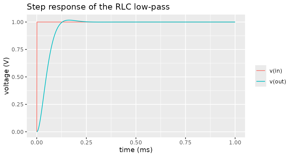
For a quick look, autoplot() draws any plot with a
scale:
autoplot(spice_plots(res)[["AC Analysis"]])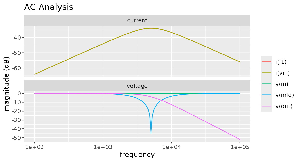
Decks as chunks
Loading spice also gives knitr a spice engine. In R
Markdown or Quarto, a ```{spice} chunk holds a deck: the
engine runs it, prints the head of its tidy table, and leaves the result
in a variable named after the chunk label, ready for the R chunks below
it (see ?spice_knitr for the chunk options).
divider
v1 1 0 dc 0
r1 1 2 1k
r2 2 0 3k
.dc v1 0 10 1
.end
#>
[38;5;246m# A tibble: 33 × 7
[39m
#>    plot                       point scale_name scale variable type    value
#>
[3m
[38;5;246m<chr>
[39m
[23m
[3m
[38;5;246m<int>
[39m
[23m
[3m
[38;5;246m<chr>
[39m
[23m
[3m
[38;5;246m<dbl>
[39m
[23m
[3m
[38;5;246m<chr>
[39m
[23m
[3m
[38;5;246m<chr>
[39m
[23m
[3m
[38;5;246m<dbl>
[39m
[23m
#>
[38;5;250m 1
[39m DC transfer characteristic     1 v(v-sweep)     0 v(1)     voltage     0
#>
[38;5;250m 2
[39m DC transfer characteristic     2 v(v-sweep)     1 v(1)     voltage     1
#>
[38;5;250m 3
[39m DC transfer characteristic     3 v(v-sweep)     2 v(1)     voltage     2
#>
[38;5;250m 4
[39m DC transfer characteristic     4 v(v-sweep)     3 v(1)     voltage     3
#>
[38;5;250m 5
[39m DC transfer characteristic     5 v(v-sweep)     4 v(1)     voltage     4
#>
[38;5;250m 6
[39m DC transfer characteristic     6 v(v-sweep)     5 v(1)     voltage     5
#>
[38;5;250m 7
[39m DC transfer characteristic     7 v(v-sweep)     6 v(1)     voltage     6
#>
[38;5;250m 8
[39m DC transfer characteristic     8 v(v-sweep)     7 v(1)     voltage     7
#>
[38;5;250m 9
[39m DC transfer characteristic     9 v(v-sweep)     8 v(1)     voltage     8
#>
[38;5;250m10
[39m DC transfer characteristic    10 v(v-sweep)     9 v(1)     voltage     9
#>
[38;5;246m# ℹ 23 more rows
[39m
autoplot(spice_plots(divider)[[1]])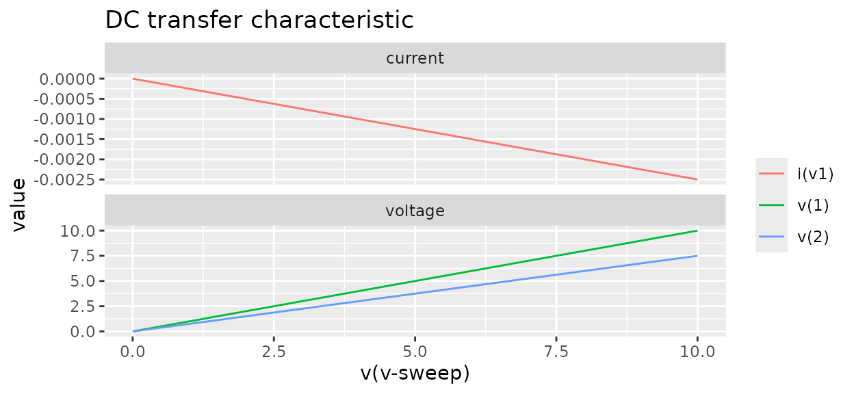
Circuits from figures
A schematic drawn in pic with the dune
prelude (resistor(), vsource(),
npn(), …; the figure opts in with spice = 1)
is a deck too: spice_pic() extracts its netlist – the block
labels are the refdes, the wires the nodes – and
spice_run() runs the extraction.
spice_pic_svg() draws the figure.
fig <- ".PS
spice = 1
In: (0,1); Out: (2,1)
V1: vsource(In, (0,0), DC 5)
R1: resistor(In, Out, 1k)
R2: resistor(Out, (2,0), 3k)
line from R2.N to V1.N; ground(V1.N)
.op
.PE"
p <- spice_pic(fig)
cat(p$netlist)
#> * netlist extracted by dune-pic
#> V1 In 0 DC 5
#> R1 In Out 1k
#> R2 Out 0 3k
#> .op
#> .end
spice_run(p) |> spice_op("out")
#> v(out)
#>   3.75
p$map$pins
#> # A tibble: 6 × 5
#>   refdes pin   net       x     y
#>   <chr>  <chr> <chr> <dbl> <dbl>
#> 1 V1     P     In        0     1
#> 2 V1     N     0         0     0
#> 3 R1     P     In        0     1
#> 4 R1     N     Out       2     1
#> 5 R2     P     Out       2     1
#> 6 R2     N     0         2     0
Exchanging rawfiles
Results write to and read from SPICE3 rawfiles, the format ngspice
reads and writes with -r:
f <- tempfile(fileext = ".raw")
spice_write_raw(res, f)
back <- spice_read_raw(f)
identical(spice_tidy(back), spice_tidy(res))
#> [1] TRUE